We’ve reached the end of the main series, so it’s time to put everything we’ve learned to good use. In this article, I’ll unveil MacroFactor’s new equations for estimating BMR, based on everything we’ve covered in this series. We’re confident that these equations will estimate BMR more accurately for more people than any other BMR equations.
We have that confidence for a few reasons:
- We’re starting from a good spot. Based on a thorough review of the research, we’re confident that the Oxford/Henry equations and the 1991 Cunningham equation are the best “off the shelf” BMR equations out there right now. They’re what we’re using to ground our new equations, which won’t deviate too far from that strong foundation.
- Both of these equations were designed to be easy to use in an era when everyone didn’t have a computer in their pocket. As a result, they don’t make use of (relatively simple) mathematical functions that are known to help with more accurately estimating BMR – especially for relatively small or relatively large people.
- There’s room to improve on these equations because they still have blind spots. The Oxford/Henry and Cunningham equations are great, but they’re not applicable to every population. For instance, they both reliably underestimate BMR in muscular athletic populations.
- There’s low-hanging fruit to pick. As we’ve discussed in this series, metabolic adaptation decreases BMR below what would be expected during weight loss, but no popular BMR equations account for it.
- Other equations that account for age do so linearly, despite the fact that BMR decreases more gradually through most of adulthood, and more aggressively past 60 years old.
So, let’s dive in.
Scaling metabolism
Way back in the first article of this series, I cited a paper by Wang and colleagues that modeled BMR as a function of fat-free mass based on relationships observed across species, and based on the scaling of organ mass with body size in humans. They found that these relationships could be approximated with linear equations that were very similar to the 1991 Cunningham equation: BMR = 21.6 × Fat-Free Mass + 370. However, the actual modeled equations were non-linear – the linear equations just served as “close enough” approximations for most people.
In the second article of this series, I cited research by Müller and colleagues, illustrating how high-metabolic-rate tissue mass scales with body size. Again, their data revealed a nonlinear relationship.
In the third article in this series, I cited research by Pontzer and colleagues, modeling how BMR scales similarly with fat-free mass in both men and women. These cutting-edge metabolism researchers also chose to model the relationship with non-linear equations.
All three of these studies reveal a well-understood principle of metabolism: metabolic rates scale allometrically.
Allometric scaling describes how various characteristics scale across organisms of different sizes, and why those scaling relationships exist. As it relates to metabolism, when organisms get larger, they tend to slow down … relatively speaking. An elephant obviously has a higher BMR than a shrew, but per unit of body mass, the elephant’s BMR is much, much, much lower. But, this decrease as organisms get larger is nonlinear, so allometric relationships are described by power law functions, rather than linear equations.
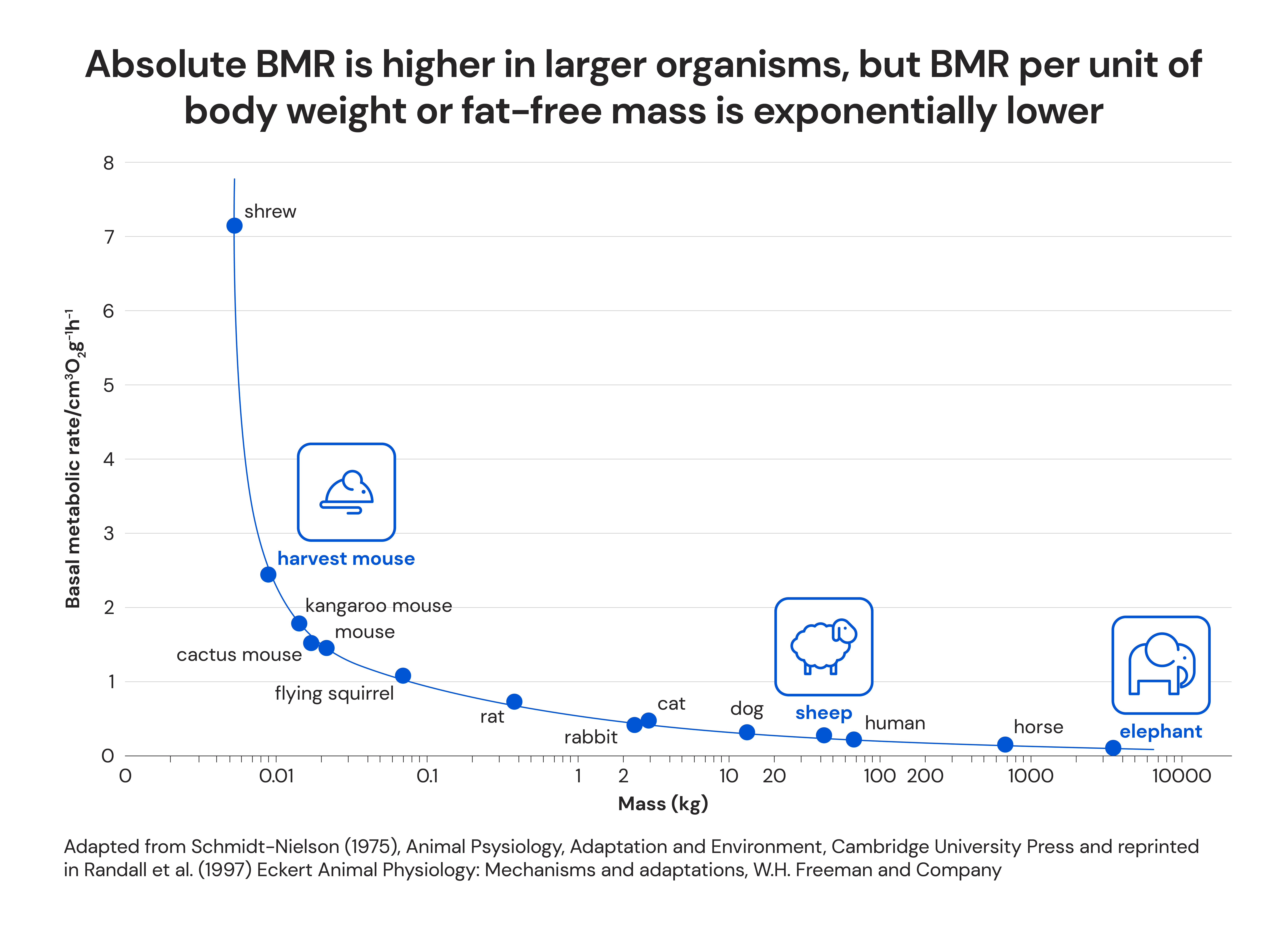
Obviously the size difference between the largest and smallest humans isn’t nearly as vast as the size difference between an elephant and a shrew, but humans do differ in size considerably. The very largest human adults are more than five times larger than the very smallest human adults. In other words, we span a large enough size range to warrant allometric scaling. Linear equations describe human metabolism well for most relatively normal-sized people, but they’ll tend to overestimate BMR for particularly small people, and particularly large people (and slightly underestimate BMR for normal-sized people).
This was perhaps best illustrated in a study by Bowes and colleagues. They analyzed the data in the Schofield/FAO database, and found that non-linear allometric equations described the relationship between body size and BMR far better than linear relationships.
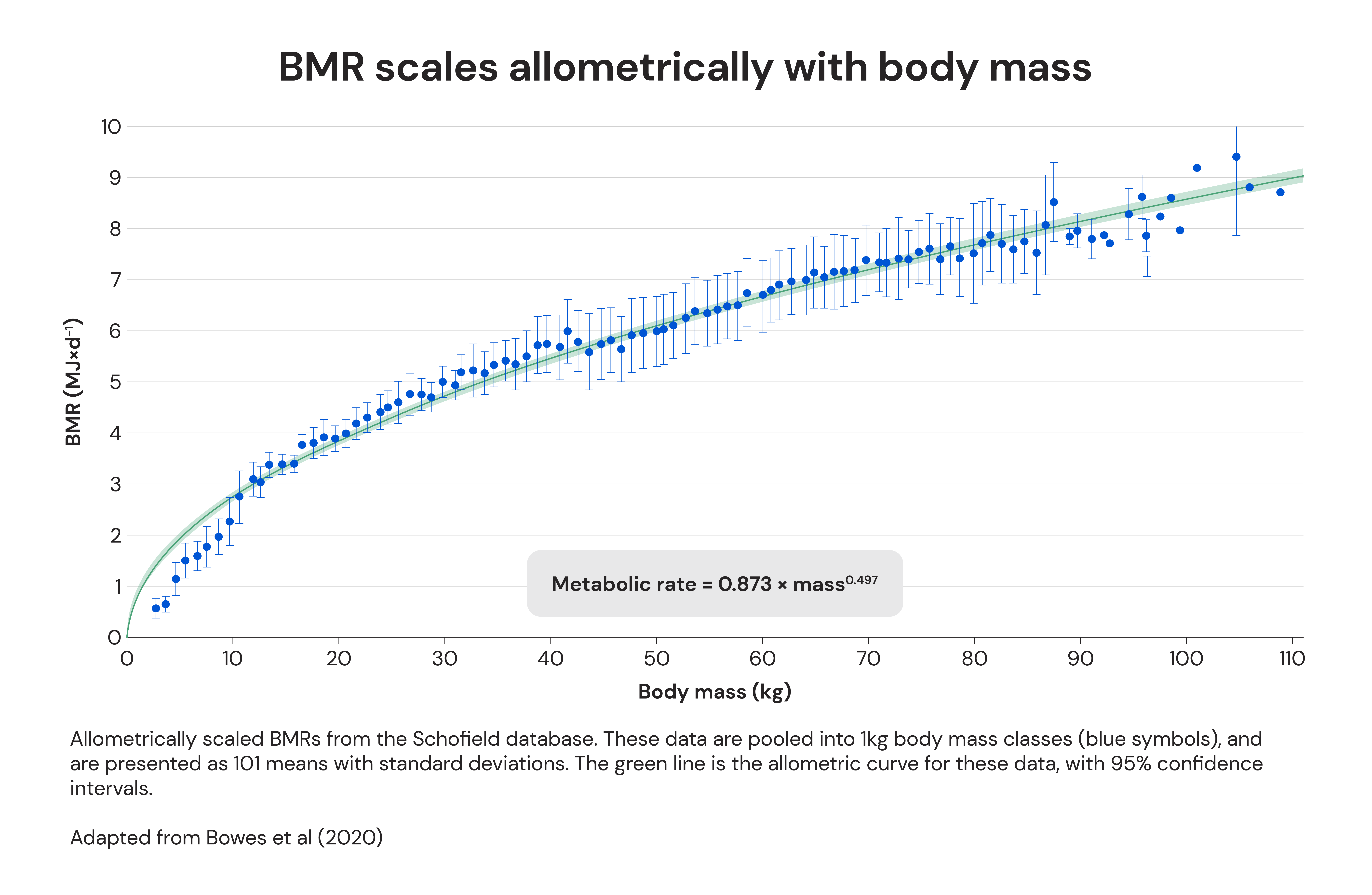
So, when modifying the Oxford/Henry equations – which predict BMR based on height, weight, age, and sex – we need to examine the allometric relationship between BMR and weight, and the allometric relationship between BMR and height. And, for modifying the Cunningham equation – which predicts BMR based on fat-free mass – we need to examine the allometric relationship between BMR and fat-free mass, and potentially consider the role of fat mass as well.
Starting with fat-free mass, the traditional view that was originally advanced by Kleiber (the founder of this field of research) is that BMR scales with fat-free mass raised to the power of 0.75. Since then, there’s been a growing contingent of researchers advocating for the perspective that BMR in humans scales with fat-free mass raised to the power of 0.66. Although I genuinely find the back-and-forth fascinating, this isn’t the time to go too far into the weeds on the topic. So, for our purposes here, I think (hope) all parties can agree that scaling to the power of 0.7 neatly splits the difference, while offering a considerable improvement over linear scaling.
Moving onto fat mass, there’s a strong case to be made for incorporating fat mass into body composition-based equations. Research indicates that people with more fat mass may have slightly more high-metabolic-rate organ mass per unit of fat-free mass. So, while fat mass itself doesn’t contribute THAT much to BMR, it’s still indicative of a shifting relationship between fat-free mass and BMR. That should be fairly intuitive if you think about it for a moment. If two people have an identical amount of fat-free mass, but one of them weighs 80kg, and the other weighs 150kg, I think we’d all expect the person who weighs 150kg to have a higher BMR. Unfortunately, there’s not as much theory to draw upon for determining the correct scaling exponent to describe the relationship between fat mass and BMR (after accounting for variation in fat-free mass), beyond saying that the effect (and therefore the exponent) should be quite small. However, a recent large study found that a scaling exponent of 0.066 worked well, and that seems like a perfectly reasonable value.
For body weight, there’s more applicable research. Researchers rarely explicitly report allometric analyses of human metabolic rates, but you can easily estimate and model the allometric relationships implied by linear BMR equations (essentially reversing the process Wang and colleagues used in their study). You can sometimes find implied scaling exponents for men that are close to 0.7, and values for women that are around 0.4. But, values of around 0.6 for men and 0.5 for women are most common. I tested the effect of using different scaling values for men and women, but the impact of using 0.6 for men and 0.5 for women wasn’t meaningfully different than just using 0.55 for both sexes. So, in the interest of parsimony, we’re going with a universal scaling exponent of 0.55. Much like the debate regarding scaling exponents between 0.66 and 0.75 for fat-free mass, any value between 0.4 and 0.7 is a clear improvement over the scaling value of 1 implied by linear equations.
Finally, height: the allometric relationship between height and BMR hasn’t received much research attention. However, we know that both total fat-free mass and high-metabolic-rate organ mass scales strongly with height – both of which are strong predictors of BMR. Fat-free mass scales with height raised to the power of approximately 2. A case could be made for using slightly different exponents for different populations, but once again, a value of 2 is a clear improvement over the value of 1 implied by linear equations.
So, rather than using linear equations, we’ll improve upon the Oxford/Henry and Cunningham equations by scaling BMR to weight raised to the power of 0.55, height raised to the power of 2, and fat-free mass raised to the power of 0.7. We’ll also include fat mass in our replacement for the Cunningham equation, scaling fat mass to the power of 0.066.
Accounting for athletes
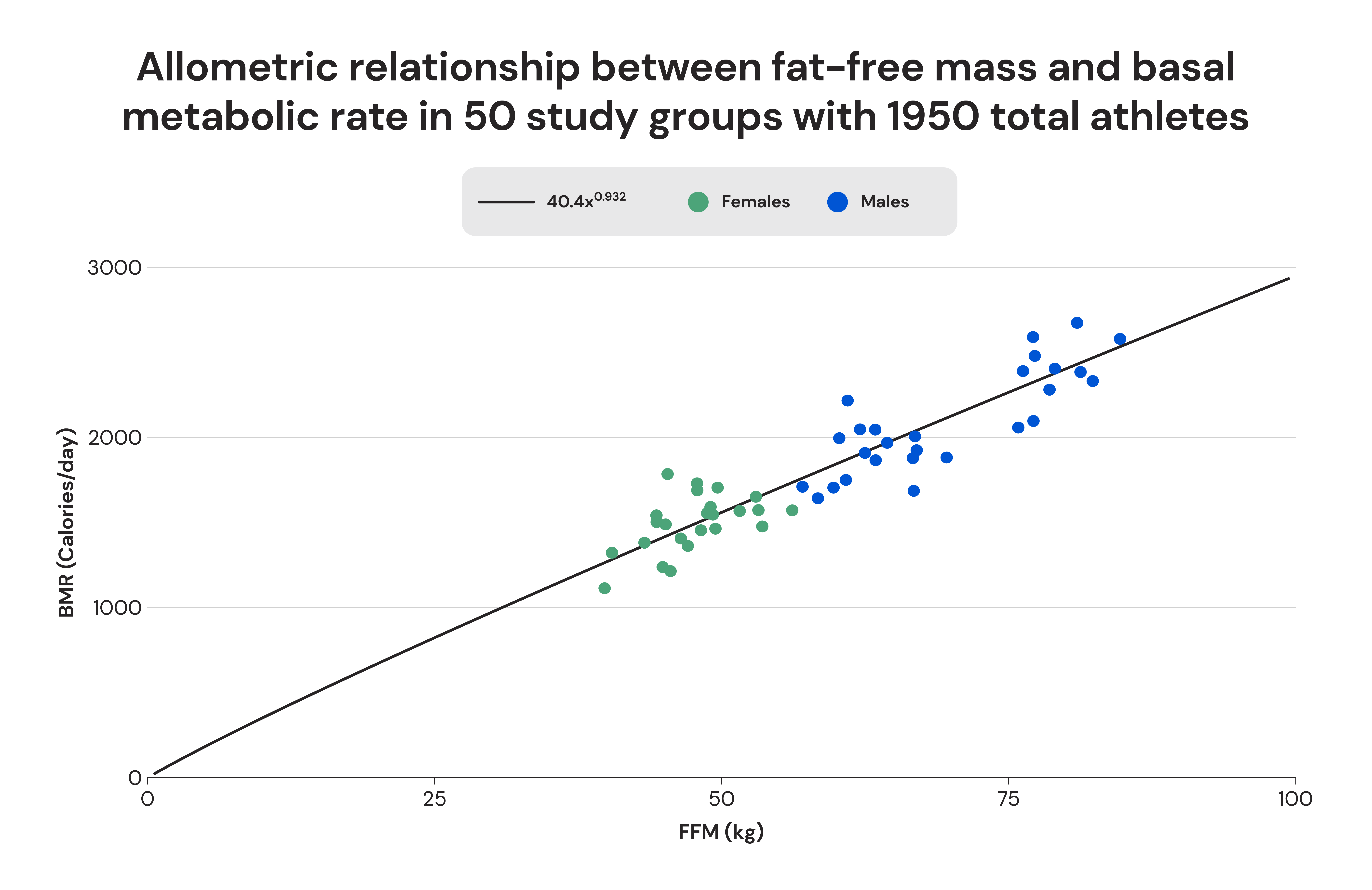
As discussed in a prior article in this series, athletes have higher BMRs per unit of fat-free mass than non-athletes. The difference grows as fat-free mass increases, primarily because athletes with large amounts of fat-free mass have larger high-metabolic rate organs than non-athletes with large amounts of fat-free mass.
Because of this, the relationship between fat-free mass and BMR follows an essentially linear relationship in athletes. When I tested an allometric relationship, the scaling exponent to describe the relationship between fat-free mass and BMR was 0.932, which is considerably higher than the values we observe in the general population.
In testing on the dataset, I also found that incorporating fat mass into the equation slightly improved model fit, but I excluded it as a term in the final equation. It seemed to only tangibly improve predictions by reducing BMR estimates for athletes who were likely underfueling to maintain particularly lean physiques; for example, the largest negative residuals in the studies I analyzed came from a study on high-level ballet dancers who were extremely lean.
Since there was only one study on older athletes in my dataset, and since the athletes in that study had BMRs that were comparable to younger athletes, I determined that there was insufficient reason and evidence to justify including an age term.
Metabolic adaptation
Our article on the impact of weight loss on BMR already covered the topic of metabolic adaptation extensively. Even though metabolic adaptation is well-understood and extensively researched, standard BMR prediction equations don’t include a term to account for it. So, factoring in the effect of metabolic adaptation is a bit of low-hanging fruit to improve the predictive accuracy of our equations.
With reasonable weight loss interventions, metabolic adaptation of about 5% is pretty typical. Furthermore, greater weight loss tends to increase metabolic adaptation, and persistent metabolic adaptation of about 3-5% seems to be fairly normal following extensive weight loss and subsequent weight maintenance.
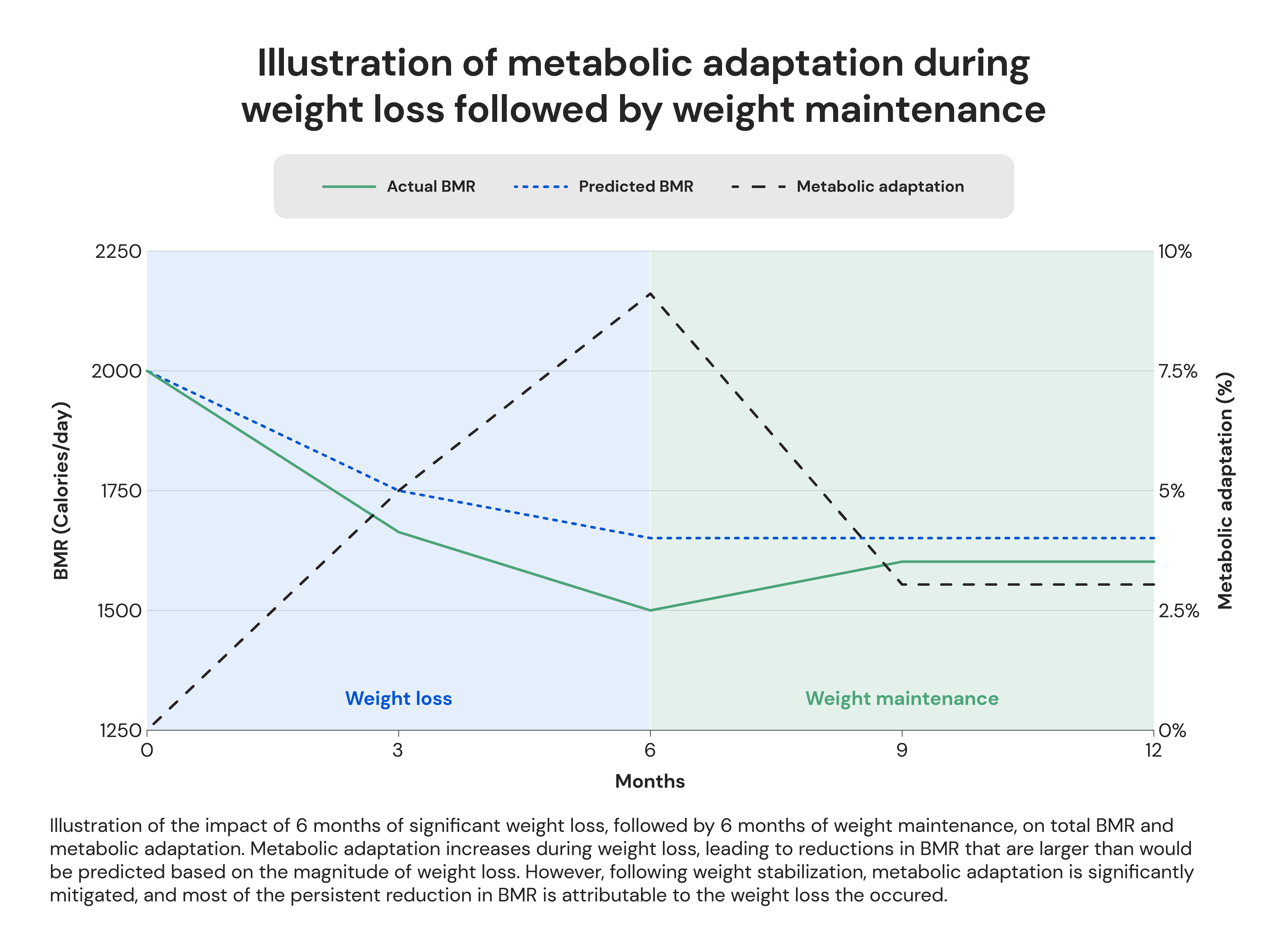
So, if you’re in an energy deficit, your predicted BMR will be 5% lower using our equations. And, if your current body weight is more than 10% below your peak body weight, your predicted BMR will be an additional 3% lower. A case could be made for more aggressive values (especially if you’re maintaining a very aggressive deficit, or getting extremely lean), but I think it’s prudent to err on the side of caution. Even conservatively accounting for metabolic adaptation is a clear improvement over not accounting for it at all, and I think the risk of erring too low (and thus accidentally recommending an energy deficit that would be far too aggressive) exceeds the risk of erring a bit high.
The non-uniform impact of age
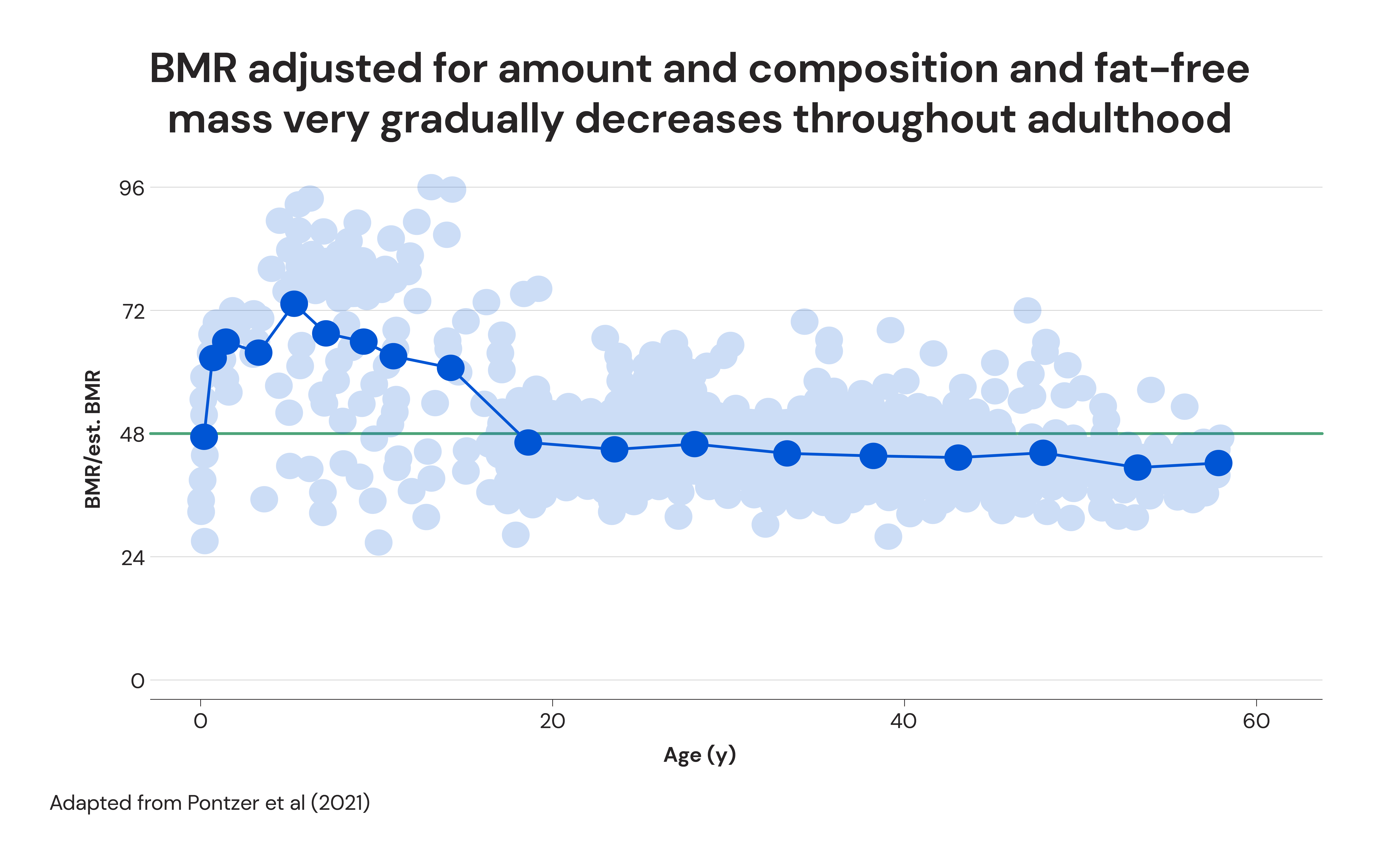
As we discussed in the fourth article in this series, BMR (adjusted for body size and body composition) decreases very gradually throughout most of adulthood. However, the rate of decline approximately doubles or triples beyond the age of 60. So, the “age” term in our formulas will reflect this fact.
Putting it all together
For modifying the Oxford/Henry and Cunningham equations, I started by calculating estimated BMRs for the participants in the NHANES body composition database. This was the largest representative dataset I could get my hands on that had body composition data for all subjects.
On average, the Oxford/Henry equations produced slightly higher BMR estimates than the Cunningham equation. Since both are high-quality equations that go about estimating BMR in slightly different ways, I averaged the estimates of the two equations for each subject (the product of two good estimates should be another good estimate), and used the resulting values as the dataset to develop new equations against. This ensures that, on average, our improved equation using height and weight, and our improved equation using fat mass and fat-free mass will produce similar BMR estimates for people with more-or-less “normal” body composition for their age, height, weight, and sex.
Our improved equation based on height, weight, age, and sex is as follows:
BMR = 129.6 × Weight0.55 + 0.011 × Height2 – [1.96;4.9] × Age – 213.8 × Sex
Weight is in kilograms, height is in centimeters, and for sex, male = 0 and female = 1. BMR is reduced by 1.96 Calories for each year up to 60 years old, and 4.9 Calories for each year past 60 years old
Our improved equation based on fat-free mass and fat mass is as follows:
BMR = 50.2 × FFM0.7 + 40.5 x (FFM0.7 × FM0.066) – [1.1;2.75] × Age
FFM = Fat-Free Mass in kg, FM = Fat Mass in kg. BMR is reduced by 1.1 Calories for each year up to 60 years old, and 2.75 Calories for each year past 60 years old
For this equation, I tested fat-free mass in isolation, fat-free mass and fat mass as independent terms, and the interaction between fat-free mass and fat mass. The prior research on the topic found that the interaction of fat-free mass and fat mass was a strong predictor, which my testing confirmed. The inclusion of allometrically scaled fat mass as an independent term didn’t improve model fit, but the combination of fat-free mass and the interaction term performed better than either term in isolation.
Our improved equation for athletes is as follows:
BMR = 40.4 × FFM0.932
FFM = Fat-Free Mass in kg
Functionally, “athlete” is defined here as anyone spending at least seven hours per week engaged in intense exercise.
Finally, adjustments for metabolic adaptation:
If you’re presently in an energy deficit, the BMR estimate is reduced by 5% to account for the impact of metabolic adaptation (i.e. the output of the formula is multiplied by 0.95). Furthermore, if your current body weight is more than 10% lower than your highest body weight, the BMR estimate is reduced by 3%. So, if you’re currently losing weight and your current weight is more than 10% lower than your highest body weight, multiply the output of the formula by 0.92. If you’re currently weight-stable or gaining weight, but your current body weight is more than 10% lower than your highest body weight, multiply the output of the formula by 0.97.
Naturally, we don’t expect you to do all of that math by hand, nor should you need to type the equations into your phone calculator. We’ve made a BMR calculator that will do all of these calculations for you, and compare the results to other popular BMR formulas. These are also the equations we’ll use to estimate your BMR (in order to initially estimate your total daily energy expenditure) in the MacroFactor app.
Looking ahead
This concludes the core of this series, but there are still a couple things to look forward to.
First, we have a couple more articles planned to round out common questions people have about BMR: one will tackle the range of human BMRs, and one will discuss whether women with PCOS have lower BMRs.
Second, we believe that these are currently the best BMR equations out there, but there’s still room for improvement. Namely, it’s high time for someone to repeat the process Cunningham carried out in 1991, and Henry carried out in 2005: the world needs another fully comprehensive review and meta-analysis of the BMR literature. We at MacroFactor will be heading up and funding that endeavor in the coming year.
Stay tuned.